- What we want to achieve
- Matlab version
- Toolbox
- Download URL
- Folder Structure
- How to run the program
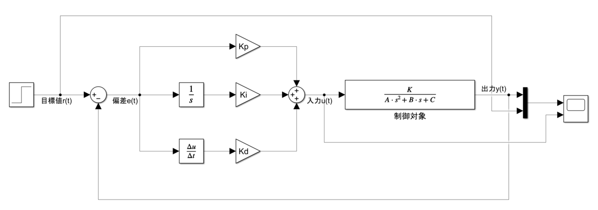
- Simulink File(PID_fmin.slx)
- m-file code (Main_PID_fmin_input.m)
- m-file code (func_fmin_input.m)
- Simulation result
- Discussions
- Recommended Past Articlesforfree.hatenablog.jp
What we want to achieve
- Construction of a PID control simulator using Simulink and m-files
- Optimization of PID gains for the above program
- Optimization using fminsearch
- Optimization to prevent excessive input
Matlab version
Matlab2021a
*Past versions also available as downloadable formats
Toolbox
Download URL
*Download the folder for the Matlab version you are using.
Example: If you are using the 2021a version, select "2021a" from the link above.
*We are not responsible for any problems caused by the use of the above programs.
Folder Structure
Download and extract the above.

How to run the program
Run "Main_PID_fmin_input.m"
Simulink File(PID_fmin.slx)
m-file code (Main_PID_fmin_input.m)
%% Initializationclc % Initialize command windowclear % Initialize workspaceclose all % Close all graphs%% Variable Declaration% ===== Controlled system =====K = 1;A = 1;B = 1;C = 1;% ===== reference signal =====r_val = 10; % step reference signal% ===== Simulink =====N_File = 'PID_fmin.slx'; % simulink filne nameFinalTime = 30; % Simulation end time [s]SamplingTime = 0.1; % Sampling time [s]% ===== Estimated system gain =====K_hat = 0.1*K; % It is used in fminsearch%% fminsearchini_x = [0.5 0.5, 0.5]; % Initial PID gains[x, fval] = fminsearch(@(x) func_fmin_input(x,N_File,K_hat),ini_x);%% Run the Simulinkopen(N_File); % Open Simulink filesim(N_File); % Run the Simulink
%% Output Figures% ===== Store the Simulink data =====t = ScopeData.time; % Timey = ScopeData.signals(1).values(:, 1); % Outputr = ScopeData.signals(1).values(:, 2); % Reference signalu = ScopeData.signals(2).values(:, 1); % Input% ===== output figures =====% ----- y -----figure;subplot(211);plot(t,y);hold on;plot(t,r,'--');grid on;xlabel('$ t {\rm [s]} $', 'interpreter', 'latex');ylabel('$ y(t) $', 'interpreter', 'latex');legend('$ y(t) $', '$ r(t) $', 'interpreter', 'latex');% ----- u -----subplot(212);plot(t,u);hold on;grid on;xlabel('$ t {\rm [s]} $', 'interpreter', 'latex');ylabel('$ u(t) $', 'interpreter', 'latex');
m-file code (func_fmin_input.m)
function f = func_fmin_input(x,N_File,K_hat)%% Variable DeclarationKp = x(1);Ki = x(2);Kd = x(3);assignin('base','Kp',Kp);assignin('base','Ki',Ki);assignin('base','Kd',Kd);% Run the Simulinksim(N_File);%% Store the Simulink datat = ScopeData.time; % Timey = ScopeData.signals(1).values(:, 1); % Outputr = ScopeData.signals(1).values(:, 2); % Reference signalu = ScopeData.signals(2).values(:, 1); % Input%% 評価規範
% To make the same order between error and input, intrduce a K_hatf = sum*1.^2);%% output optimization results in command windowfprintf('[Kp, Ki, Kd, fval] = %.3g, %.3g, %.3g, %.3g\n',Kp, Ki, Kd, f);
Simulation result
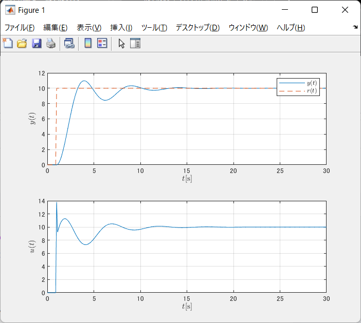
Discussions
【Objective function】
where is the estimated system gain,
is the input value in steady state.
Recommended Past Articlesforfree.hatenablog.jp
*1:r-y).^2 + (K_hat.*(u(end)-u